
This post is part of Oracle SQL tutorial and we would be discussing Analytic functions in oracle(Over by partition) with examples, detailed explanation .
Analytic functions in oracle
We have already studied about Oracle Aggregate function like avg ,sum ,count. Lets take an example
First lets create the sample data
CREATE TABLE "DEPT"
( "DEPTNO" NUMBER(2,0),
"DNAME" VARCHAR2(14),
"LOC" VARCHAR2(13),
CONSTRAINT "PK_DEPT" PRIMARY KEY ("DEPTNO")
)

CREATE TABLE "EMP"
( "EMPNO" NUMBER(4,0),
"ENAME" VARCHAR2(10),
"JOB" VARCHAR2(9),
"MGR" NUMBER(4,0),
"HIREDATE" DATE,
"SAL" NUMBER(7,2),
"COMM" NUMBER(7,2),
"DEPTNO" NUMBER(2,0),
CONSTRAINT "PK_EMP" PRIMARY KEY ("EMPNO"),
CONSTRAINT "FK_DEPTNO" FOREIGN KEY ("DEPTNO")
REFERENCES "DEPT" ("DEPTNO") ENABLE
);

SQL> desc emp
Name Null? Type
---- ---- -----
EMPNO NOT NULL NUMBER(4)
ENAME VARCHAR2(10)
JOB VARCHAR2(9)
MGR NUMBER(4)
HIREDATE DATE
SAL NUMBER(7,2)
COMM NUMBER(7,2)
DEPTNO NUMBER(2)

SQL> desc dept
Name Null? Type
---- ----- ----
DEPTNO NOT NULL NUMBER(2)
DNAME VARCHAR2(14)
LOC VARCHAR2(13)


insert into DEPT values(10, 'ACCOUNTING', 'NEW YORK');
insert into dept values(20, 'RESEARCH', 'DALLAS');
insert into dept values(30, 'RESEARCH', 'DELHI');
insert into dept values(40, 'RESEARCH', 'MUMBAI');
commit;

insert into emp values( 7839, 'Allen', 'MANAGER', 7839, to_date('17-11-1981','dd-mm-yyyy'), 20, null, 10 );
insert into emp values( 7782, 'CLARK', 'MANAGER', 7839, to_date('9-06-1981','dd-mm-yyyy'), 0, null, 10 );
insert into emp values( 7934, 'MILLER', 'MANAGER', 7839, to_date('23-01-1982','dd-mm-yyyy'), 0, null, 10 );
insert into emp values( 7788, 'SMITH', 'ANALYST', 7788, to_date('17-12-1980','dd-mm-yyyy'), 800, null, 20 );
insert into emp values( 7902, 'ADAM, 'ANALYST', 7832, to_date('23-05-1987','dd-mm-yyyy'), 1100, null, 20 );
insert into emp values( 7876, 'FORD', 'ANALYST', 7566, to_date('3-12-1981','dd-mm-yyyy'), 3000, null, 20 );
insert into emp values( 7369, 'SCOTT', 'ANALYST', 7566, to_date('19-04-1987','dd-mm-yyyy'), 3000, null, 20 );
insert into emp values( 7698, 'JAMES', 'ANALYST', 7788, to_date('03-12-1981','dd-mm-yyyy'), 950, null, 30 );
insert into emp values( 7499, 'MARTIN', 'ANALYST', 7698, to_date('28-09-1981','dd-mm-yyyy'), 1250, null, 30 );
insert into emp values( 7844, 'WARD', 'ANALYST', 7698, to_date('22-02-1981','dd-mm-yyyy'), 1250, null, 30 );
insert into emp values( 7654, 'TURNER', 'ANALYST', 7698, to_date('08-09-1981','dd-mm-yyyy'), 1500, null, 30 );
insert into emp values( 7521, 'ALLEN', 'ANALYST', 7698, to_date('20-02-1981','dd-mm-yyyy'), 1600, null, 30 );
insert into emp values( 7900, 'BLAKE', 'ANALYST', 77698, to_date('01-05-1981','dd-mm-yyyy'), 2850, null, 30 );
commit;
Now the example of aggregate functions will be given as below
select count(*) from EMP;
---------
13

select sum (bytes) from dba_segments where tablespace_name='TOOLS';
-----
100

SQL> select deptno ,count(*) from emp group by deptno;

DEPTNO COUNT(*)
---------- ----------
30              6
20              4
10              3
Here we can see that it reduces the number of rows in each of the queries. Now questions comes what to do if we need to have all the rows returned with count(*) also
For that oracle has provided a sets of analytic functions. So to solve the last problem , we can write as
select empno ,deptno , count(*) over (partition by deptno) from emp group by deptno;
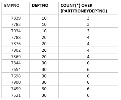
Here count(*) over (partition by dept_no) is the analytical version of the count aggregate function. The main key work which is different by aggregate function is over partition by
Analytic functions compute an aggregate value based on a group of rows. They differ from aggregate functions in that they return multiple rows for each group. The group of rows is called a window and is defined by the analytic_clause.
General Syntax for Analytic functions
Here is the general syntax
analytic_function([ arguments ]) OVER ([ query_partition_clause ] [ order_by_clause [ windowing_clause ] ])
Example
count(*) over (partition by deptno)

avg(Sal) over (partition by deptno)
Lets go over each part
query_partition_clause
It defined the group of rows. It can like below
partition by deptno : group of rows of same deptno
or
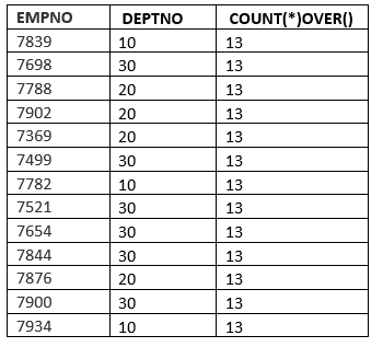
() : All rows
SQL> select empno ,deptno , count(*) over () from emp;
[ order_by_clause [ windowing_clause ] ]
This clause is used when you want to order the rows in the partition. This is particularly useful if you want analytical function to consider the order of the rows.
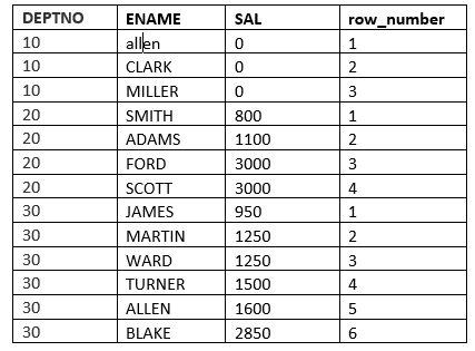
Example will be row_number function
SQL> select
deptno, ename, sal,
 row_number() over (partition by deptno order by sal) "row_number" from emp;
Another example would be
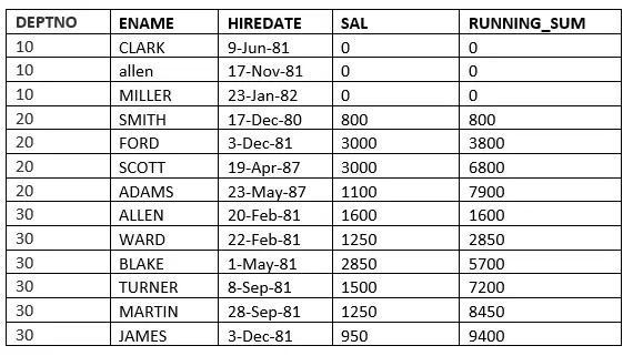
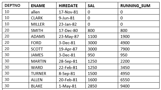
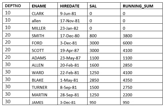
SQL> select deptno, ename,hiredate, sal,sum(sal) over (partition by deptno order by HIREDATE) running_sum from emp;
Windowing_clause
This is always used with order by clause and give more control over the set of the rows in the group
With Windowing clause, For each row, a sliding window of rows is defined. The window determines the range of rows used to perform the calculations for the current row. Window sizes can be based on either a physical number of rows or a logical interval such as time.
When using order by clause and nothing is given for windowing_clause,below default value of the windowing_clause is taken
RANGE BETWEEN UNBOUNDED PRECEDING AND CURRENT ROW or RANGE UNBOUNDED PRECEDING
It means “The current and previous rows in the current partition are the rows that should be used in the computation”
The example below clearly states this. This goes the running average in the department
SQL> select deptno, ename,hiredate, sal,sum(sal) over (partition by deptno order by HIREDATE) running_sum from emp;

Now windowing_clause can be defined with number of ways
Lets first understand the terminology
ROWS specifies the window in physical units (rows).
RANGE specifies the window as a logical offset. the RANGE windowing clause can be used only with ORDER BY clauses containing columns or expressions of numeric or date datatypes
PRECEDING – get rows before the current one.
FOLLOWING – get rows after the current one.
UNBOUNDED – when used with PRECEDING or FOLLOWING, it returns all before or after. CURRENT ROW
Types of Windowing clause
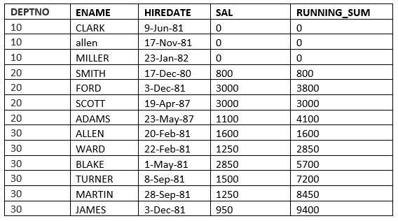
ROWS UNBOUNDED PRECEDING : The current and previous rows in the current partition are the rows that should be used in the computation
SQL> select deptno, ename,hiredate, sal,sum(sal) over (partition by deptno order by HIREDATE ROWS UNBOUNDED PRECEDING) running_sum from emp;

RANGE UNBOUNDED PRECEDING : The current and previous rows in the current partition are the rows that should be used in the computation. Also since range is specified ,it all takes those values which are equal to the current rows.
SQL> select deptno, ename,hiredate, sal,sum(sal) over (partition by deptno order by HIREDATE RANGE UNBOUNDED PRECEDING) running_sum from emp;

You may not see the difference between range and rows as hire_date is different for all.The difference will become more clear if we use sal as order by clause
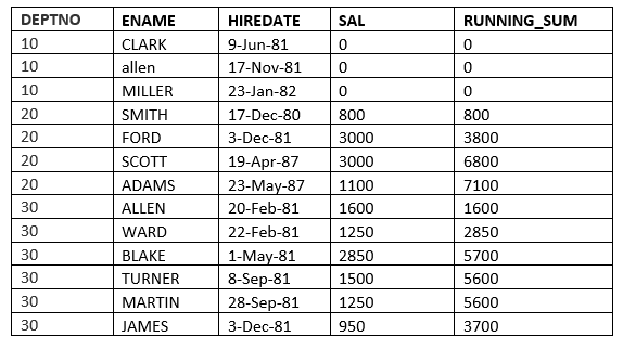
SQL> select deptno, ename,hiredate, sal,sum(sal) over (partition by deptno order by sal RANGE UNBOUNDED PRECEDING) running_sum from emp;

SQL> select deptno, ename,hiredate, sal,sum(sal) over (partition by deptno order by sal ROWS UNBOUNDED PRECEDING) running_sum from emp;
You can find the difference on line 6
RANGE value_expr PRECEDING : The window begins with the row whose ORDER BY value is numeric expression rows less than, or preceding, the current row and ends with the current row being processed.
SQL> select deptno, ename,hiredate, sal,sum(sal) over (partition by deptno order by HIREDATE RANGE 365 PRECEDING) running_sum from emp;
Here it takes all the rows where hiredate value falls within 365 days preceding the hiredate value of the current row
ROWS value_expr PRECEDING : The window begins with the row given and ends with the current row being processed
SQL> select deptno, ename,hiredate, sal,sum(sal) over (partition by deptno order by HIREDATE ROWS 2 PRECEDING) running_sum from emp;
Here the window start from 2 rows preceding the current row
RANGE BETWEEN CURRENT ROW and value_expr FOLLOWING : The window begins with the current row and ends with the row whose ORDER BY value is numeric expression rows less than, or following
SQL> select deptno, ename,hiredate, sal,sum(sal) over (partition by deptno order by HIREDATE ROWS between current row and 1 FOLLOWING) running_sum from emp;
ROWS BETWEEN CURRENT ROW and value_expr FOLLOWING : The window begins with the current row and ends with the rows after the current one
SQL> select deptno, ename,hiredate, sal,sum(sal) over (partition by deptno order by HIREDATE ROWS between current row and 1 FOLLOWING) running_sum from emp;
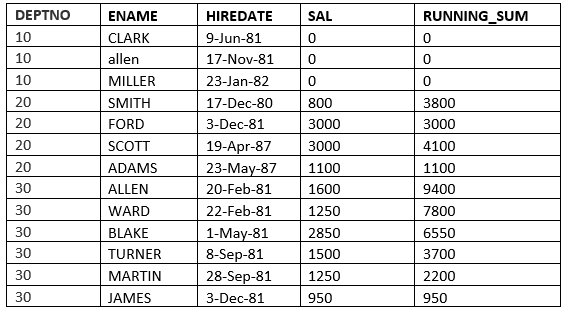
RANGE BETWEEN UNBOUNDED PRECEDING and UNBOUNDED FOLLOWING
SQL> select deptno, ename,hiredate, sal,sum(sal) over (partition by deptno order by HIREDATE RANGE BETWEEN UNBOUNDED PRECEDING and UNBOUNDED FOLLOWING
) running_sum from emp;

RANGE BETWEEN value_expr PRECEDING and value_expr FOLLOWING
SQL> select deptno, ename,hiredate, sal,sum(sal) over (partition by deptno order by HIREDATE RANGE BETWEEN 365 PRECEDING and 365 FOLLOWING
) running_sum from emp; 2

DEPTNO       ENAME      HIREDATE      SAL      RUNNING_SUM
---------- ---------- --------------- ---------- -----------
10           CLARK       09-JUN-81      0          0
10           ALLEN       17-NOV-81      0          0
10           MILLER      23-JAN-82      0          0
20           SMITH       17-DEC-80      800       3800
20           FORD        03-DEC-81      3000      3800
20           SCOTT       19-APR-87      3000      4100
20           ADAMS       23-MAY-87      1100      4100
30           ALLEN       20-FEB-81      1600      9400
30           WARD        22-FEB-81      1250      9400
30           BLAKE       01-MAY-81      2850      9400
30          TURNER       08-SEP-81      1500      9400
30          MARTIN       28-SEP-81      1250      9400
30          JAMES        03-DEC-81      950       9400

13 rows selected.
Some Important Notes
(1)Analytic functions are the last set of operations performed in a query except for the final ORDER BY clause. All joins and all WHERE, GROUP BY, and HAVING clauses are completed before the analytic functions are processed. Therefore, analytic functions can appear only in the select list or ORDER BY clause.
(2)Analytic functions are commonly used to compute cumulative, moving, centered, and reporting aggregates.
I hope you like this detailed explanation of Analytic functions in oracle(over by Partition Clause)
Related Articles
LEAD Function in Oracle
DENSE function in Oracle
Oracle LISTAGG Function
Aggregating Data Using Group Functions
https://docs.oracle.com/cd/E11882_01/server.112/e41084/functions004.htm