Microsoft Excel is used by almost everybody. Here are some of the cool Excel features that everybody should be aware
- Using Excel function to complete many tasks
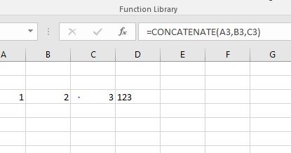
Excel has a powerful list of functions to solve various problems and tasks. You can use sum, concatenate, average, if. The list goes on
2) Auto Filter
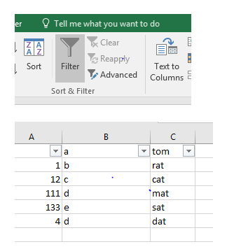
This is one of the best functions to use when playing with a lot of data in Excel. You can filter any column and find the corresponding intersection very easily.
Just go to the top and click on filter, and your Excel sheet will converted into filter form as shown below.
3) Conditionally Format
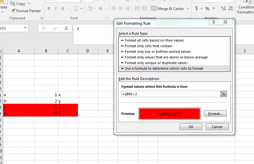
We may be asked many times to present the data in such a form so that highlights are visible like Who has the highest (or lowest) sales, what the top five are, etc.. Excel’s Conditional Formatting will do everything from putting a border around the highlights to colour-coding the entire table. Use the Highlighted Cells Rules sub-menu to create more rules to look for things, such as text that contains a certain string of words, recurring dates, duplicate values, etc. There’s even a greater than/less than option so you can compare number changes.
The simple operation is shown below, We colored the row where the E column is greater than 2
4) Great Excel Shortcut Keys
| CNTRL B | Insert the current time (the colon is what is in a clock reading, like 12:00). |
| CNTRL -k | Add Hyperlink |
| CNTRL- S | Save the file |
| CNTRL -1 | Format the cell |
| CTRL+SHIFT+L | Turn on/off the filter |
| F12 | Save as |
| CNTRL + F2 | Print preview |
| Shift + F11 | Add new sheet |
| ALT+ ENTER | Get a line break inside the cell |
| CNTRL+F4 | Close the workbook |
| Ctrl+; | Inserts today’s date. |
| Ctrl+Shift+: | Inserts the current time (the colon is what is in a clock reading, like 12:00). |
| Ctrl+0 | Hides the current column |
| Ctrl+9 | Hides the current row |
| Ctrl+F6 | Switches between open workbooks (that is, open Excel files in different windows). |
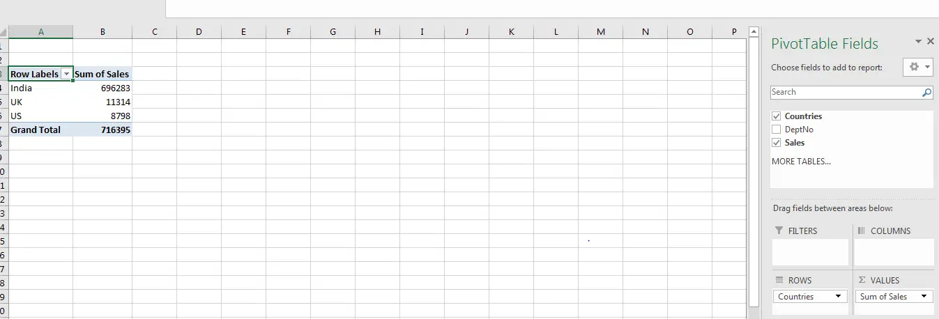
5) Pivot Table
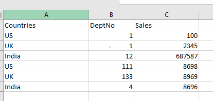
It is also one of the powerful features in Microsoft Excel to analyze and present the data
If you have well-organized source data, you can create a pivot table in less than a minute. Here’s how:
1. Select any cell in the source data
2. On the Insert tab of the ribbon, click the PivotTable button
3. In the Create PivotTable dialog box, check the data and click OK
4. Drag a “label” field into the Row Labels area
Example
6) Using Macros
you can automate tasks in Excel by writing so-called macros. First, we need to enable the developer toolbar to do it
Each Excel version has different ways to enable the developer toolbar
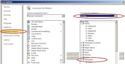
Excel 2010
In Excel 2010 you can display the developer toolbar in the following way:
- Click the green File Button
- Press Options
- Make sure that the Customize Ribbon right menu item is selected.
- In the dropdown list called Customize the Ribbon, select All Tabs.
- In the group called Main Tabs, make sure that the option Developer is checked.
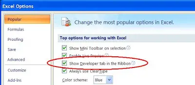
Excel 2007
To display the developer ribbon, do the following:
- Click the Office Button
- Click the Excel Options button at the bottom of the dialog.
- Ensure that the Popular tab in the left menu is selected (se picture below)
- Check the option Show Developer tab in the Ribbon
Now once the developer toolbar is visible , we can record any macro and then use it
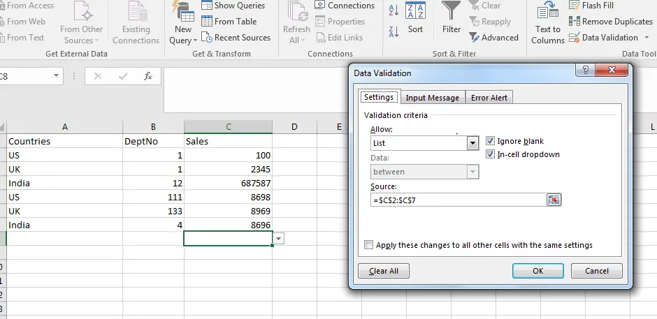
7) Validate Data to Make Drop Downs
If you Creating a spreadsheet for others to use and wants that people should enter some valid values only then it will be beneficial to create a drop-down menu of selections to use in particular cells (so they can’t screw it up!), that’s easy. We can create this using the below steps
- Highlight the cell, go to the Data tab, and click Data Validation.
- Under “Allow:” select “List.”
- Then in the “Source:” field, type a list, with commas between the options. Or, you could click the button next to the Source field and go back into the same sheet to select a data series
- You can hide that data later, it’ll still work.
Example
Hope you like these cool Excel features and use them in your daily tasks. Please do provide feedback